AMI SQL

Goals

The 3Forge SQL language provides a comprehensive instruction set for working with table(s) of data.

• Retrieval - Accessing and Normalizing data from external sources
• Blending - Perform Joins and Unions on tables
• Modifying - Inserting, Updating, and Deleting rows
• Analyzing - Grouping, Sorting, and Filtering
• Schema Definition - Creating, Updating, and Dropping tables

Broadly speaking, the logic steps involved in data-visualization are:

1. Running a query, or set of queries, on external datasources and/or the AMI-Realtime database.

• Each datasource is predefined and uniquely named.
• The results of queries on datasources will result in temporary, in-memory tables
• The queries can be constructed using user-input/user-selected/user-associated data
• In more advanced cases, the queries can be sequential, meaning the results from one query are then fed into a subsequent query (allowing for reactionary data blending)

2. Blending the results from Step 1, resulting in new temporary in-memory tables 3. Building visualizations on the tables from Step 1 and/or Step 2

AMI SQL and Standard SQL Differences

For those familiar with standard SQL, these are the differences:

1. Equality is done with ==

• AMISQL: SELECT * FROM Users WHERE userid == 15;
• MYSQL: SELECT * FROM Users WHERE userid = 15;

2. Checking for null is done with equality, ex. == null

• AMISQL: SELECT * FROM Users WHERE status == null;
• MYSQL: SELECT * FROM Users WHERE status IS NULL;

3. Strings are surrounded in double quotes

• AMISQL: SELECT * FROM Users WHERE name == "David";
• MYSQL: SELECT * FROM Users WHERE name = "David";

4. "Matches" (~~) instead of LIKE

• AMISQL: SELECT * FROM Users WHERE name ~~ "^Dav";
•  MYSQL: SELECT * FROM Users WHERE name LIKE "Dav%";

 (See Simplified Text Matching for pattern matching rules/expressions)

5. Boolean expressions && works same as AND.  || works same as OR

• AMISQL: SELECT * FROM Users WHERE userid == 15 AND status == null && name == "David";
• MYSQL: SELECT * FROM Users WHERE userid = 15 AND status IS NULL && name = "David";

6. By default all tables are TEMPORARY, use the PUBLIC key word to make non-temporary tables:

• AMISQL: CREATE TABLE MyTemporaryTable(id String);
• AMISQL: CREATE PUBLIC TABLE MyPermanantTable(id String);

Data Source Access Clauses

use...execute_clause

Overview

This command enables you to "execute" code on an external datasource and process/store the results locally

• USE: While datamodels have default options, you can override them for a particular query.  Valid options include
  • ds = "datasource_name"
    • The name of the datasource to execute this script on
  • timeout = timeout_in_millis
    • The number of milliseconds before the execute command times out
  • limit = row_limit_to_return
    • The max number of records returned
  • ds_url = "url"
    • Overrides the url of the datasource
    • When used in conjunction with ds="datasource_name", supplied datasource must contain URL in the PermittedOverrides field
  • ds_username = "username"
    • Overrides the username of the datasource
    • When used in conjunction with ds="datasource_name", supplied datasource must contain USERNAME in the PermittedOverrides field
  • ds_password = "plain_text_password"
    • Overrides the password of the datasource using a plain text password
    • When used in conjunction with ds="datasource_name", supplied datasource must contain PASSWORD in the PermittedOverrides field
    • Mutually exclusive with the ds_password_enc option
  • ds_password_enc = "aes_encrypted_password"
    • Overrides the password of the datasource, using an encrypted password
    • Use strEncrypt(...) to create an encrypted password
    • When used in conjunction with ds="datasource_name", supplied datasource must contain PASSWORD in the PermittedOverrides field
    • Mutually exclusive with the ds_password option
  • ds_options = "some options"
    • Override the options of the datasource
    • When used in conjunction with ds="datasource_name", supplied datasource must contain OPTIONS in the PermittedOverrides field
  • ds_relay = "relayid"
    • Override the relay of the datasource
    • Run SHOW RELAYS command and inspect RelayId for available relays
    • When used in conjunction with ds="datasource_name", supplied datasource must contain RELAY in the PermittedOverrides field
  • ds_adapter = "SOME_ADAPTER"
    • Use an "anonymous" datasource of the specified adapter type
    • Run SHOW DATASOURCE_TYPES command and inspect the I column for available adapters
    • Mutually exclusive with ds="datasource_name" option
    • See ami.db.anonymous.datasources.enabled option for permission details
  • _custom=some_directive
    • Prefixing with an underbar (_) passes the option through to the datasource's adapter
• EXECUTE: The literal text to execute. The text will be sent directly to the datasource for execution. Therefore, variables cannot be referenced. Instead, substitution can be used. See dollarsign_substitution

Syntax

[USE option = value  [  option = value  ...]]  EXECUTE code_to_execute

Example

CREATE TABLE

 final_table AS

USE

 ds="mydb"

 timeout=10000

 limit=100

EXECUTE

 select * from mytable;

use...show tables clause

Overview

This command enables you to see what tables are available on a given datasource (similar to what the AMI gui wizard shows you when selecting a table).

• USE: While datamodels have default options, you can override them for a particular query.  Valid options include
  • ds = "datasource_name"             The name of the datasource to execute the script on

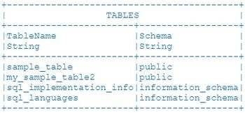
The resulting table will be called TABLE and contain two String columns: TableName and Schema

Syntax                                                                                                  

USE ds="mydb" SHOW TABLES;

Example

This example will return a table displaying all tables available in the mydb datasource. If the datasource supports schema names, that will be populated as well.

USE ds="mydb" SHOW TABLES;

//returns:

use...insert clause

Overview

This command uploads data from AMI into a datasource.

• USE: While datamodels have default options, you can override them for a particular query.  Valid options include
  • ds = "datasource_name"             The name of the datasource to execute the script on

The resulting table will be called TABLE and contain two String columns: TableName and Schema

Syntax

USE ds="datasource_name"  INSERT [INTO] datasource_table  [(col1[, col2 ...])] select_clause
USE ds="datasource_name"  INSERT [INTO] datasource_table  [(col1[, col2 ...])] analyze_clause 
USE ds="datasource_name"  INSERT [INTO] datasource_table  [(col1[, col2 ...])] prepare_clause 
USE ds="datasource_name"  INSERT [INTO] datasource_table  [(col1[, col2 ...])] execute_clause
USE ds="datasource_name"  INSERT [INTO] datasource_table  [(col1[, col2 ...])] VALUES values_expr[, values_expr ...]
USE ds="datasource_name"  INSERT [INTO] datasource_table  [(col1[, col2 ...])] Use_execute_clause

datasource_name - string name of the datasource containing the table to insert values into

datasource_table - name of the table to insert values into

Examples

This example will insert two rows into the mydb datasource's users table:

USE ds="mydb" INSERT INTO users(name,city,state) values ("Rob","NYC","NY"),("Sara","OC","CA");

This example copy all rows from AMI's my_users table into the "mydb" datasource's users table:

USE ds="mydb" INSERT INTO users(name,city,state) SELECT Name,Local,Region FROM my_users;

This example copy all rows from the old_users table in the otherds datasource to the users table in the mydb datasource.

USE ds="mydb" INSERT INTO users(name,city,state) USE ds="otherds" EXECUTE SELECT * FROM old_users

concurrent_block (advanced)

Overview

When running analysis that needs to query many datasources, there can be large performance gains by executing these queries simultaneously. The CONCURRENT{...} key word causes all EXECUTE clauses within the block to be run in parallel (instead of sequentially).

In both of the examples below, we are going to execute three queries on three separate datasources (mydb1, mydb2, mydb3). The first example executes the queries sequentially and the second example executes the queries concurrently.

Assuming each query takes 2 seconds for a database to process, the first example will complete in about 6 seconds (2+2+2), while the second, concurrent, example will complete in only 2 seconds:

Example of Sequential Execution (Default)

{
  CREATE TABLE mytable1 AS USE ds="mydb1" EXECUTE select * from mytable;
  CREATE TABLE mytable2 AS USE ds="mydb2" EXECUTE select * from mytable;
  CREATE TABLE mytable3 AS USE ds="mydb3" EXECUTE select * from mytable;
}

Here is the sequence of events:

00:00:00 -  EXECUTE clause is sent to mydb1

00:00:00 -  AMI Script sleeps until there is a response from mydb1...

00:00:02 - mytable1 is created (from result of query to mydb1)

00:00:02 -  EXECUTE clause is sent to mydb2

00:00:02 -  AMI Script sleeps until there is a response from mydb2...

00:00:04 - mytable2 is created (from result of query to mydb2)

00:00:04 -  EXECUTE clause is sent to mydb3

00:00:04 -  AMI Script sleeps until there is a response from mydb3...

00:00:06 - mytable3 is created (from result of query to mydb3)

00:00:06 -  Block is complete after 6 seconds (code after the block will be executed)

Example of Concurrent Execution

So now let's add the CONCURRENT keyword before the block.  In this case, all 3 executes will be initiated at the same time.

CONCURRENT{
  CREATE TABLE mytable1 AS USE ds="mydb1" EXECUTE select * from mytable;
  CREATE TABLE mytable2 AS USE ds="mydb2" EXECUTE select * from mytable;
  CREATE TABLE mytable3 AS USE ds="mydb3" EXECUTE select * from mytable;
}

Here is the sequence of events:

00:00:00 - EXECUTE clause is sent to mydb1

00:00:00 - EXECUTE clause is sent to mydb2

00:00:00 - EXECUTE clause is sent to mydb3

00:00:00 - AMI Script sleeps until there is a response from all 3 queries...

00:00:02 - mytable1 is created (from result of query to mydb1)

00:00:02 - mytable2 is created (from result of query to mydb2)

00:00:02 - mytable3 is created (from result of query to mydb3)

00:00:02 -  Block is complete after 2 seconds (code after the block will be executed)

Query Clauses

select_clause

Overview

This clause allows the combination of Filtering (WHERE), Sorting (ORDER BY), Aggregating (GROUP BY), Projecting (SELECT …) and Cropping (LIMIT) of individual tables.  Next, the results may be combined via Unions (UNION) and/or Joins (FROM … JOIN ON). Complex Strings containing delimited data can be split into distinct rows via the UNPACK operation. Finally, see the create_table_as_clause for storing the final result of a select clause into another table.

• To aggregate data, use the GROUP BY clause to identify any number of columns or derived values that should be used to group rows. Provide an alias (AS) for derived values to be used within the select clause. The select columns can only use aggregate functions (min, max, count, sum) on underlying rows and columns declared in the group-by clause
• To filter data, provide a WHERE clause which evaluates to a Boolean.  True indicates don't filter. When filtering in conjunction with aggregating (GROUP BY), those records filtered out will not be considered for aggregation.  To filter rows after aggregation, use the HAVING clause.
• For projecting, supply columns to include in the SELECT clause.  Derived values may be provided. Provide an alias (AS) for derived values or to rename a column.  Use star (*) to include all columns or tblname.* to include only those columns from a particular table provided in the FROM clause.
• To crop out rows, use the LIMIT clause. You may provide a number of rows to skip (offset) and a number of maximum rows to return (rowcount).
• To sort, use the ORDER BY clause. If multiple expressions are given the left-most takes priority.
• To union (concatenate) the results from multiple select clauses, use the UNION clause. The column names and types from the first select clause will provide the result set schema definition.  All select clauses participating in a union must define the same number of columns. Note: this operates like a union all in many databases.
• To join (blend) tables, supply all tables together in the FROM clause and a Cartesian product will be provided. For more advanced Joins, you can use a combination of the LEFT, RIGHT, OUTER, JOIN, ON and NEAREST clauses. See JOINING DATA section for details
• To process String columns containing multi-value delimited data, use the UNPACK col ON delimeter expression. This will split the string such that each entry will result in a new row.

Syntax

SELECT column_expr|lambda_expr  [,  column_expr|lambda_expr  ...] FROM table_expr|nested_select_expr  [, table_expr|nested_select_expr  ...]|
    [[LEFT|RIGHT|OUTER] [ONLY] JOIN [table_expr|nested_select_expr] [ON expr] [NEAREST nearest_expr]]
    [WHERE where_expr ]
    [GROUP BY column_expr [, column_expr ...] [HAVING expr ]]
    [ORDER BY expr [ASC|DESC] [, expr [ASC|DESC] ...]]
    [UNPACK col_to_unpack ON unpack_delimiter [,col_to_unpack ON unpack_delimiter]]
    [LIMIT [offset,] rowcount]
[UNION select_clause] 

offset - integer number of rows to skip

rowcount - integer number of maximum rows that will be returned

Joining Data

Simple Cartesian Joins

Any number of tables can be joined by simply listing them after the FROM clause which will produce a Cartesian product, such that a row will be returned for each possible combination of rows from the source table.  For example, the Cartesian product of a table with 5 rows and another table with 3 rows will produce 15 rows (5x3=15). Of course, the WHERE clause can be used to limit results to only the interesting combinations.

Handling Rows that don't match rows in other tables

For more granular control when joining two tables, use the JOIN syntax.  There are 7 types of statements, let's assume two tables a and b:

• FULL JOIN: FROM a JOIN b ON expr - This is the same as FROM a,b WHERE expr
• LEFT JOIN: FROM a LEFT JOIN b ON expr - A FULL JOIN plus all records from table a that would otherwise be omitted (due to the expr).
• LEFT ONLY JOIN: FROM a LEFT ONLY JOIN b ON expr - Includes only records from table a that would otherwise be omitted (due to the expr).
• RIGHT JOIN: FROM a RIGHT JOIN b ON expr - A FULL JOIN plus all records from table b that would otherwise be omitted (due to the expr). (similar to LEFT JOIN, swapping a and b)
• RIGHT ONLY JOIN: FROM a RIGHT ONLY JOIN b ON expr - Includes only records from table b that would otherwise be omitted (due to the expr). (similar to LEFT ONLY JOIN, swapping a and b)
• OUTER JOIN: A FULL JOIN plus all records from table a and from table b that would otherwise be omitted (due to the expr
• OUTER ONLY JOIN: Includes only records from table a and from table b that would otherwise be omitted (due to the expr).

Joining to a nearest match

Use the NEAREST clause in conjunction with one of the above 7 JOIN clauses to match two records where there may not be an exact match, such as doing an "as-of" join with timestamps. After the ON clause, include a NEAREST fuzzy_clause.

Consider: a JOIN b ON on_expr NEAREST fuzzy_clause, where the fuzzy clause is one of the 5 syntaxes:

• a.cola == b.colb - For each row in table a, join with the row in table b that satisfies on_expr and has the smallest delta between cola and colb.
• a.cola <= b.colb - For each row in table a, join with the row in table b that satisfies on_expr and cola is less than or equal to colb and has the smallest delta between cola and colb.
• a.cola >= b.colb - For each row in table a, join with the row in table b that satisfies on_expr and cola is greater than or equal to colb and has the smallest delta between cola and colb.
• a.cola < b.colb - For each row in table a, join with the row in table b that satisfies on_expr and cola is less than colb and has the smallest delta between cola and colb.
• a.cola > b.colb - For each row in table a, join with the row in table b that satisfies on_expr and cola is greater than colb and has the smallest delta between cola and colb.

Note the ordering of table a vs b in the fuzzy_clause does not matter. For example  b.colb >= a.cola is the same as a.cola <= b.colb

General Examples

SELECT age, dob, weight, name FROM Patients
SELECT age, dob, weight, name FROM Patients WHERE name =~ "mr"
SELECT count(*) as cnt, age, avg(dob), stdev(weight) FROM Patients GROUP BY age ORDER BY age
SELECT * FROM Patients, Accounts WHERE Patients.id == Accounts.patient_id
SELECT * FROM Orders JOIN MarketData ON Orders.symbol==MarketData.symbol NEAREST marketData.time<=Orders.time
SELECT * EXCEPT (OrderID, Quantity) from Orders; //return all Orders data except the OrderID and Quantity Columns
SELECT * FROM Orders where OrderId in ("a1","a2","b1");
SELECT * FROM Orders where OrderId in (select origOrderId from AnotherTable);
SELECT * FROM Orders where (OrderId, account) in (("a1","account1"),("a2","account1"),("b1","account2"));
SELECT * FROM Orders where (OrderId, account) in (select origOrderId, origAccount from AnotherTable);
SELECT DISTINCT EXAMPLE
SELECT symbol FROM MarketData GROUP BY symbol; //Get unique symbols from the MarketData table.

Nearest Join Examples

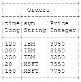
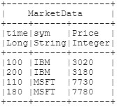
//Assume two existing tables: Orders and MarketData

AMIDB> SELECT * FROM Orders;

AMIDB> SELECT * FROM MarketData;

//A JOIN will only include orders that have a satisfactory market data event. Note, we’re also calculating the price delta from the order vs the market

AMIDB> select *,Orders.Price-MarketData.Price as delta from Orders JOIN MarketData ON Orders.sym==MarketData.sym NEAREST Orders.time>=MarketData.time ORDER by Orders.time;

//A LEFT JOIN will include all orders, event those without a market data event (using null as a place holder).

AMIDB> select *,Orders.Price-MarketData.Price as delta from Orders LEFT JOIN MarketData ON Orders.sym==MarketData.sym NEAREST Orders.time>=MarketData.time ORDER by Orders.time;

Join Examples

Let's assume we have two tables A and B, each with 1 column:

We can see that the value 1 only exists in the A table, the value 3 exists only in the B table and the value 2 existing in both tables.  When comparing the data between them there are, exhaustively speaking, 7 different ways you could want to see what matches and what doesn't.

	JOIN	OUTER JOIN	OUTER ONLY JOIN	LEFT JOIN	LEFT ONLY JOIN	RIGHT JOIN	RIGHT ONLY JOIN
Include Matches?	YES	YES		YES
Includes Left W/O a Match on Right		YES	YES	YES	YES
Includes Right W/O a Match on Left		YES	YES			YES	YES

JOIN Syntax - Return only those rows with values that coexist in both tables.  (Note, this is the same as the natural join select * from a,b where a.aid==b.bid)

SELECT * FROM a JOIN b on a.aid==b.bid

OUTER JOIN Syntax - Return all rows from both tables.

SELECT * FROM a OUTER JOIN b on a.aid==b.bid

OUTER ONLY JOIN Syntax - Return rows in the left table that don't have matching rows in the right table and rows in the right table that don't have matching rows in the left table.

SELECT * FROM a OUTER ONLY JOIN b on a.aid==b.bid

LEFT JOIN Syntax - Return all rows from the left table and only the rows in the right table matching rows in the left table.

SELECT * FROM a LEFT JOIN b on a.aid==b.bid 

LEFT ONLY JOIN Syntax - Return only rows in the left table that don't have matching rows in the right table.

SELECT * FROM a LEFT ONLY JOIN b on a.aid==b.bid 

RIGHT JOIN Syntax - Return all rows from the right table and only the rows in the left table matching rows in the right table.  (Note, this is equivalent to … FROM b LEFT JOIN a …)

SELECT * FROM a RIGHT JOIN b on a.aid==b.bid 

RIGHT ONLY JOIN Syntax - Return only rows in the right table that don't have matching rows in the left table.  (Note, this is equivalent to … FROM b LEFT ONLY JOIN a …)

SELECT * FROM a RIGHT ONLY JOIN b on a.aid==b.bid 

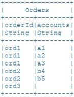
Unpack example

CREATE TABLE Orders (orderId String,accounts String);
INSERT INTO Orders VALUES("ord1","a1,a2,a3"),("ord2","b4,b5"),("ord3","");
SELECT * FROM Orders UNPACK accounts ON ",";

analyze_clause

Overview

This command runs analysis on a table. Analysis is performed on rows contained in a defined window, similar to a self-join. Each window can define an order-by to allow for finer control over the order in which an aggregate is applied.  Multiple windows may be defined. See window_expr in nested expressions for details.

When adding columns, the new cells will default to null. The column will be added to the end (right-most) of the table.

ANALYZE agg_expr [, agg_expr ...]  FROM tblname  window_expr  [,  window_expr  ...]

tblname - string name of the table to alter the schema of

Example

CREATE TABLE
  final_table AS
ANALYZE
  a_date AS date,
  BETA(win.a_open, win.b_open) AS beta,
  COR(win.a_open, win.b_open) AS cor
FROM source_table
WINDOW
  win ON win.date <= date + __date_range && date <= win.date

prepare_clause

Overview

This command allows the user to "prepare" additional columns whose values are calculated as aggregates across rows. For example, a running sum needs to consider not just the current row, but all rows before the current row. This can be accomplished using the STACK() method inside a PREPARE clause (see example below).

• ORDER BY: In many cases, the ordering of rows in the input table is important, especially for running sums. The ORDER BY clause is useful to guarantee the correct ordering.
• PARTITION BY: Used to perform many aggregates on a single table, each aggregate considering only a subset of the table's rows based on some grouping criteria.

PREPARE prep_expr [, prep_expr ...]  FROM tblname   
  [ORDER BY expr [ASC|DESC] [, expr [ASC|DESC] ...]]
  [PARTITION BY column_expr [, column_expr ...]

tblname - string name of the table to alter the schema of

Example

This example will produce a running sum of the qty column order by extime on a per-account basis

CREATE TABLE
  final_table AS
PREPARE account, qty, extime, STACK(qty) as acc_qty FROM table ORDER BY extime
PARTITION BY account

Data Modification

insert_values_clause

Overview

This clause enables the insertion of raw values into an existing table.  Many rows may be inserted in a single call. Each values_expr represents a single row of data to be inserted. To insert multiple rows append additional values_expr

In order to specify columns in which to insert values, provide an ordered list of column names after the table name.  The same number of values must be supplied in the values_expr and in the same order.  All other columns will default to null.

If a list of column names is not provided, all columns will be populated. Each values_expr should contain one value for each column in the target table. Values should be in the same natural order as the columns in the target table.

The forloop_expr allows for the insertion of values_expr to be repeated for each cycle of the for loop. The values can reference the for loop's declared variable. Multiple for loops can be nested inside one another.

Syntax

INSERT [INTO]  tblname [(col1[, col2 ...])] [forloop_expr ...] VALUES values_expr[, values_expr ...] [LIMIT maxinsert]

tblname - string name of the table to insert into

colN - string name of the column to contain the Nth value from values_expr